This project saves pictures from various cameras in its pouch! The possum uses a web browser as a control panel. Since we'll be using this when travelling, it's designed to work well with Safari running on iPhone or iPodTouch. Hardware consists of a Raspberry Pi, an external hard drive, and an Edimax Wi-Fi dongle. You'll need a USB hub and a 5V power supply for both the Pi and the external hard drive.
To use the Possum, connect a camera to the hub, web into the Possum, and start backing up your pictures!
This entry describes setting up the Pi operating system and networking.
Step one was to get the pi image onto the sd card. We had started this project and made lots of progress, so I tried to clone - with no success - the image from one 4GB card to another using "dd". Every thing I tried - various block sizes of bs=4GB to bs=4GB. Every time I tried, "out-file" ran out of room.
I gave up and downloaded a fresh Raspbian image, and used Win32DiskImager to download the image (I was getting tired of "dd"). Interestingly the ras-pi web page uses a SHA-1 has to verify the integrity of the image, and Win32DiskImager only calculates MD5. That's OK. I'm living dangerously.
Since this Pi had already been on my network I knew the IP address. Time to connect.
ssh 192.168.0.204 -l pi
And I get this.
@@@@@@@@@@@@@@@@@@@@@@@@@@@@@@@@@@@@@@@@@@@@@@@@@@@@@@@@@@@
@ WARNING: REMOTE HOST IDENTIFICATION HAS CHANGED! @
@@@@@@@@@@@@@@@@@@@@@@@@@@@@@@@@@@@@@@@@@@@@@@@@@@@@@@@@@@@
IT IS POSSIBLE THAT SOMEONE IS DOING SOMETHING NASTY!
Someone could be eavesdropping on you right now (man-in-the-middle attack)!
It is also possible that a host key has just been changed.
The fingerprint for the ECDSA key sent by the remote host is
f9:4f:ab:1a:0d:cd:42:0a:7d:f7:95:5c:48:77:69:13.
Please contact your system administrator.
Add correct host key in /home/tester/.ssh/known_hosts to get rid of this message.
Offending ECDSA key in /home/tester/.ssh/known_hosts:1
remove with: ssh-keygen -f "/home/tester/.ssh/known_hosts" -R 192.168.0.204
ECDSA host key for 192.168.0.204 has changed and you have requested strict checking.
Host key verification failed.
That's because I've had one NIC with different disk image. I ran
ssh-keygen -f "/home/tester/.ssh/known_hosts" -R 192.168.0.204
And I'll use the combine the .old file to so I can run this board with either disk image.
Now log in as "pi" again, and use the password "raspberry".
Run the setup. Configure the device not to start the desktop automatically.
sudo raspi-config
Then configure the network by editing the interfaces file.
pi@raspberrypi /etc/network $ cat interfaces
auto lo
iface lo inet loopback
iface eth0 inet dhcp
auto wlan0
allow-hotplug wlan0
iface wlan0 inet dhcp
wpa-scan-ssid 1
wpa-ap-scan 1
wpa-key-mgmt WPA-PSK
wpa-proto RSN WPA
wpa-pairwise CCMP TKIP
wpa-group CCMP TKIP
wpa-ssid "mynetwork"
wpa-psk "mywpa2passphrase"
iface default inet dhcp
Starting out in infrastructure mode is handy, but the goal is to have an adhoc network so we can connect anywhere. Here's the configuration for that.
pi@raspberrypi /etc/network $ cat interfaces
auto lo
iface lo inet loopback
iface eth0 inet dhcp
allow-hotplug wlan0
iface wlan0 inet static
address 169.254.1.1
netmask 255.255.0.0
wireless-channel 6
wireless-essid mynetwork
wireless-mode ad-hoc
wireless-key 4142434445464748494a4b4c4d
There are a couple of interesting things here. First I've manually configured an auto-IP address or 169.254.1.1 which is not normally done. Since this is an ad-hoc network with no DHCP server, devices that join are supposed to auto-IP; that is, will assign themselves a random address after checking that the address isn't already taken. However, in this case, we have to know where to point our browser, so I've statically assigned it to 169.254.1.1 so we can always find it. At some point I'll look into Link Local Multicast Name Resolution (LLMNR).
The other interesting thing is the wireless key. It's a needs to be a string of 26 hexadecimal digits. When connecting to the network you don't enter these hex digits, but rather the ASCII equivalent. It this case, the key is a 13 character string: "ABCDEFGHIJKLM".

"To invent, you need a good imagination and a pile of junk." -Thomas A. Edison
Thursday, May 8, 2014


Sunday, May 4, 2014
Getting Google Maps Markers onto a Garmin eTrex GPS
To get a Google Maps marker or two onto an eTrex GPS, you can use the Garmin Communicator plug-in if you can run Internet Explorer. However, it's tedious to use when you have a large number of markers. And, what about those of us on Linux? GPSPrune did the trick for me. I was able to get GPSPrune from the Ubuntu repository using apt-get.
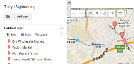
After you've created a map in Google Maps, the next step in the marker transfer process is to get the markers onto your local drive in a format recognized by GPSPrune. Click the folder icon in the upper left hand corner of your map and select "Export to KML".
Plug your GPS into the USB port and power it up. Next is a critical step that took me a while to figure out. The GPSPrune application needs access to the USB port. You could bring up a terminal and type "sudo GPSPrune" to run as super user; but don't do that. Here's the right way. Most of the info on how get GPSPrune talking to the Garmin came from this page: http://wiki.openstreetmap.org/wiki/USB_Garmin_on_GNU/Linux
First, from the console, add your user to the lp group.
sudo adduser <my_user> lp
Next type:
lsusb -v | more
This will get you information on your GPS:
Bus 005 Device 004: ID 091e:0003 Garmin International GPS (various models)
Now create and edit a USB permissions rules file.
sudo nano /etc/udev/rules.d/51-garmin.rules
And then input and save the following vendor and product IDs along with the new access mode.
ATTRS{idVendor}=="091e", ATTRS{idProduct}=="0003", MODE="666"
To activate the changes run:
sudo udevadm control --reload-rules
From GPSPrune, click File, Open File, and select your KML file. All your markers should appear. Now click File, Send Data to GPS. Uncheck "Send Tracks", then click OK.
The markers should appear on your GPS as waypoints. Here's the amazing thing about it. The marker field in Google Maps is much longer that the eTrex waypoints string. Either GPSPrune or GPSBabel (which does some of the behind-the-scenes work) abbreviates everything intelligently. For example, "Center" becomes "CNTR". I didn't need to shorten any strings beforehand.
Once I figured it out, it was a pretty easy and quick process.
After you've created a map in Google Maps, the next step in the marker transfer process is to get the markers onto your local drive in a format recognized by GPSPrune. Click the folder icon in the upper left hand corner of your map and select "Export to KML".
Plug your GPS into the USB port and power it up. Next is a critical step that took me a while to figure out. The GPSPrune application needs access to the USB port. You could bring up a terminal and type "sudo GPSPrune" to run as super user; but don't do that. Here's the right way. Most of the info on how get GPSPrune talking to the Garmin came from this page: http://wiki.openstreetmap.org/wiki/USB_Garmin_on_GNU/Linux
First, from the console, add your user to the lp group.
sudo adduser <my_user> lp
Next type:
lsusb -v | more
This will get you information on your GPS:
Bus 005 Device 004: ID 091e:0003 Garmin International GPS (various models)
Now create and edit a USB permissions rules file.
sudo nano /etc/udev/rules.d/51-garmin.rules
And then input and save the following vendor and product IDs along with the new access mode.
ATTRS{idVendor}=="091e", ATTRS{idProduct}=="0003", MODE="666"
To activate the changes run:
sudo udevadm control --reload-rules
The markers should appear on your GPS as waypoints. Here's the amazing thing about it. The marker field in Google Maps is much longer that the eTrex waypoints string. Either GPSPrune or GPSBabel (which does some of the behind-the-scenes work) abbreviates everything intelligently. For example, "Center" becomes "CNTR". I didn't need to shorten any strings beforehand.
Once I figured it out, it was a pretty easy and quick process.
Monday, November 4, 2013
More Image Sharpness
ImageMagick has FFT build into it! You just use the appropriate command line options in ImageMagic's Convert application. I found ImageMagick's FFT documentation really helpful in understanding 2d FFTs of images. I just takes two command lines. The first performs the FFT and creates a magnitude and a phase plot.
convert ohelo.png -fft fft_ohelo.png
The phase plot's not really useful to us, so we'll just take the magnitude plot, which is the one that has a -0 appended to its name. Because it's plotted on a linear scale, it doesn't look like much - almost entirely black. But if we auto-scale it, and plot logarithmically, a pattern emerges.
convert fft_ohelo-0.png -auto-level -evaluate log 10000000 fft_ohelo_10000000.png
You may have to play around with the log scaling. It took me several tries to get something usable.
Here is the set of test images:
It's hard to tell the difference between the original and the 5 pixel blur, but look at the FFTs.
The white areas farther from the center have the highest spatial frequencies and therefore are the sharpest. Blurring the image filters those out and results in a smaller circle. I'm not sure I understand the horizontal and vertical artifacts, but I think that may have something to do with the rectangular arrangement of the pixels.
To make this more quantifiable, I next plan to use ImageMagic's Sample option to grab radial lines at 5 degree increments between 5 and 85 degrees. Because of the symmetry of the quadrants, it's only necessary to sample from one of them. I'll then average the samples and plot them on an X-Y axis.
Also, to make this real, I need to take the pictures with two different cameras or lenses. I think the subject should be something natural like leaves because man-made objects in some examples I've seen tend to have strong diagonal artifacts.
A later post will explore some of these refinements and possibly add some Ruby automation to the process.
convert ohelo.png -fft fft_ohelo.png
The phase plot's not really useful to us, so we'll just take the magnitude plot, which is the one that has a -0 appended to its name. Because it's plotted on a linear scale, it doesn't look like much - almost entirely black. But if we auto-scale it, and plot logarithmically, a pattern emerges.
convert fft_ohelo-0.png -auto-level -evaluate log 10000000 fft_ohelo_10000000.png
You may have to play around with the log scaling. It took me several tries to get something usable.
Here is the set of test images:
 |
| Straight Out of the Camera |
 |
| 5 Pixel Blur |
 |
| 25 Pixel Blur |

 |
| Straight Out of the Camera |
 |
| 5 Pixel Blur |
 |
| 25 Pixel Blur |
To make this more quantifiable, I next plan to use ImageMagic's Sample option to grab radial lines at 5 degree increments between 5 and 85 degrees. Because of the symmetry of the quadrants, it's only necessary to sample from one of them. I'll then average the samples and plot them on an X-Y axis.
Also, to make this real, I need to take the pictures with two different cameras or lenses. I think the subject should be something natural like leaves because man-made objects in some examples I've seen tend to have strong diagonal artifacts.
A later post will explore some of these refinements and possibly add some Ruby automation to the process.


Sunday, November 3, 2013
How Sharp is That Lens?
As I read reviews of photographic equipment, I find the occasionally come across a review in which the reviewer notes that the reviewed lens was a dud and didn't focus properly. How could I tell if I had a dud lens without a way to compare it to others? Some kind of quantitative method for lens comparison is needed. There are all kinds of sharpness test patterns, but none of them seemed to be easy-to-use. Then I saw an example of a pattern of black and white bars that got progressively closer together. You can tell how sharp the lens is by looking at where the bars mush together to form gray. I looked at this and realized that this is the spacial equivalent of the swept-sine frequency response test used for audio equipment. What if I approached this like a signal processing problem? A basic test of signal processing equipment is the step-response. On a first-order system you can use this to determine its time constant, which is a fundamental metric. This could be the metric I was looking for? I used a laser printer to make a sheet of paper that was half black and white. I took three pictures with an old point and shoot camera: wide, tele, and purposely blurred. The photos were taken at maximum resolution.


WIDE

TELE

BLUR

Sampling a line pixels from left to right in the middle each image should result in a step response from black to white. To extract the pixel values I used a Ruby script with RMagick:
require 'RMagick'
include Magick
puts ARGV[0]
image = ImageList.new(ARGV[0])
midPointY = image.rows / 2
(0..image.columns).each do |x|
pixel = image.pixel_color(x,midPointY )
print x
print ", "
print (pixel.red + pixel.green + pixel.blue) / 3
print "\n"
end
include Magick
puts ARGV[0]
image = ImageList.new(ARGV[0])
midPointY = image.rows / 2
(0..image.columns).each do |x|
pixel = image.pixel_color(x,midPointY )
print x
print ", "
print (pixel.red + pixel.green + pixel.blue) / 3
print "\n"
end
RMagick is so cool! I sent the output of the file to a spreadsheet to compare the three images.

Look at this! The wide angle has the fastest rise time. You can even see a little 2nd order ringing that's probably due to the compression algorythm. Interestingly there's pre-ringing too because spacial systems are non-causal.
Note that the wide angle is not sharper because it had to be closer to the paper to fill the frame. I've noticed that this 12 year-old camera is just not as sharp on the telephoto setting as it used to be. This graph quantified my observation. How much of a difference is there between wide and tele? We'll zoom in on the data.


In a first-order system, the time constant is measured at 63% of the final value of the step function. There are a couple of sample points in that area, so I'll use those as an approximation rather than interpolating an exact point. Now we can say that the wide-angle setting is more than twice as sharp as the telephoto setting.
There are still some questions I'd like to answer. How can I compare cameras with different pixel resolution? Can I harmonize my results somehow with the lensmakers' specs? Could I perform an average of successive images to get a better accuracy? How could I compare the center of the lens to the edges? Would deconvolution or FFT be useful analysis tools? These are all questions for a later blog post!
Saturday, November 2, 2013
Transcription Controller in an Afternoon
I have some audio files that I need to transcribe. I figured it would be easy just to load them up in the Audacity audio editor and type away. Not so easy. People talk much faster than I can type, and it's hard to control Audacity while trying to type on the word processor. Fortunately, Audacity has keyboard short-cuts. I just need a way to connect a foot pedal to Audacity.
An old PS2 mouse makes a decent foot pedal. I gutted the unit, removing the scroll wheel, and then wired the mouse buttons to the I/O cable.

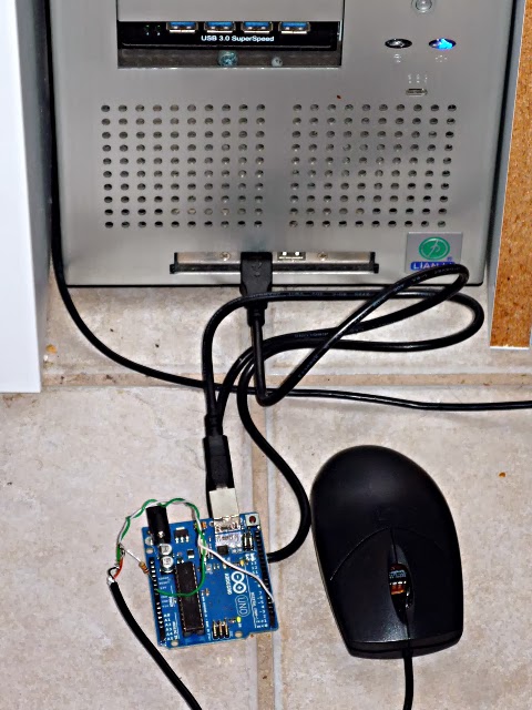
I then cut off the PS2 connector, and wired it to pin 2 of an Arduino. I also added a 10K pull-up resistor. Here's what it looks like assembled and connected.
The Arduino was programmed to send the following text strings:
15 seconds after boot: "g"
mouse down: "0"
mouse up: "1"
Here's the code (adapted from Arduino Playground):
// digital pin 2 has a pushbutton attached to it.
int pushButton = 2;
// the setup routine runs once when you press reset:
void setup() {
// initialize serial communication at 9600 bits per second:
Serial.begin(9600);
// make the pushbutton's pin an input:
pinMode(pushButton, INPUT);
delay(15000);
}
void loop() {
Serial.println("g");
int initButtonState=digitalRead(pushButton);
//loop forever
while(1)
{
// read the input pin:
int buttonState = digitalRead(pushButton);
if(initButtonState != buttonState)
{
// print out the state of the button:
Serial.println(buttonState);
//debounce
delay(5);
}
initButtonState=buttonState;
}
}
I decided to code this in Python because it's a pretty fun and easy language with lots of libraries. But, the first thing I needed was X-windows automation and there seem to be a lot of choices. Even though it's been replaced by Xaut, I found Xautomation worked for me. I got Python and Xautomation from the Linux Mint Software Library, but I could have got them as easily using apt-get.
For each of the received characters I used Xautomation to sent the following key strokes.
g = space p (start playback and pause)
0 = p (un-pause)
1 = comma comma comma comma comma p (back up a little, then pause)
The last link was the serial link connecting the Arduino to the Python code. pySerial looked like a good library, and to get it I would need python-pip.
sudo apt-get install python-pippip pySerial
pySerial didn't work at first. I found I had to execute the following commands.
sudo usermod -a -G dialout tester
sudo chmod 777 /dev/ttyACM0
The first command gives you permission to access serial I/O. The second gives you permission to use the particular USB device. Unless you have put these settings in a bash script, you'll have to execute them every time you run the program. Also, depending on your hardware, your USB device may have a different name (like ttyUSB0). The short-cut way to getting pySerial working would be to run Python as root, which is a very bad idea, however.
Here's the code with all in all its ugliness:
# serial_read_keys.py
import time
import serial
from subprocess import Popen, PIPE
control_f4_sequence = '''keydown Control_L
key F4
keyup Control_L
'''
shift_a_sequence = '''keydown Shift_L
key A
keyup Shift_L
'''
initialize_sequence = '''key space
key P
'''
play_sequence = '''key space
'''
unpause_sequence = '''key P
'''
pause_sequence = '''key P
'''
backup_sequence = '''key comma
'''
def keypress(sequence):
p = Popen(['xte'], stdin=PIPE)
p.communicate(input=sequence)
ser = serial.Serial('/dev/ttyACM0',9600)
while (1) :
#print 'reading line'
rcvChar = ser.readline()
# print rcvChar
if 'g' in rcvChar :
print 'initialize - play and pause'
keypress(play_sequence)
time.sleep(0.1)
keypress(pause_sequence)
if '0' in rcvChar :
print 'unpause'
keypress(unpause_sequence)
if '1' in rcvChar :
print 'backup a little then pause'
keypress(backup_sequence)
time.sleep(0.1)
keypress(backup_sequence)
time.sleep(0.1)
keypress(backup_sequence)
time.sleep(0.1)
keypress(backup_sequence)
time.sleep(0.1)
keypress(backup_sequence)
time.sleep(0.1)
keypress(pause_sequence)
I had to do some experimentation, and I left all of that in there so I could document what I had learned.
To do transcription, first open your audio file with Audacity. You may want to use the Effect, Change Tempo menu item to slow down the play-back. Now start the Python script. You have 15 seconds to do the following: make sure the Audacity stop button is clicked, then click on the waveform you want to transcribe.
After 15 seconds, the script will click the play button then immediately click pause. Don't touch anything on your screen again. If you do, it will lose focus and the key-presses won't go to Audacity. So, how are you supposed to type the transcription then? Use another computer! I neglected to tell you that, didn't I?
Go to the other computer, mash down on the mouse with you foot and the audio will begin to play. Release the mouse and the audio will back up about 5 seconds and then pause. Why does it back up before pausing? So you can more easily sync up your typing. If you want to back up more double click the mouse.
One unexpected nice feature I found is that when you start the script, it reboots the Arduino, so you don't have to reach down and press the reset button.
Sunday, October 27, 2013
Quantitative Analysis of My Photographic Style
I'm starting to look for a new camera. I'm moving from an advanced point-and-shoot to a basic DSLR. Choosing a body is hard enough. But, what about lenses? The answer different for everyone. It depends upon your style. Do you shoot landscapes, portraits, wildlife, or macro? I currently have a Canon S3 IS super-zoom which does fairly well at any of these, but mostly I like landscapes. Presumably I should be using wider angle settings. I'm now looking at ultra-wide zooms, but does my picture taking history show that this is the range of focal lengths that I use would use most?
First I gathered all the photos I took with my S3 on a 2010 trip to Japan. Using ExifTool, I extracted the focal length setting from every photo I took with that camera. Alternatively I might have decided to analyze only my favorite photos, but I decided to look at the larger data set. On my computer, I opened a terminal and moved to the folder containing the photos to be analyzed. It this case the photos were on a SAMBA file server. In Linux, the SAMBA path can be pretty long. I learned that you can just type "cd " in the terminal, then drag the network photos folder in the Nemo file browser to the text window to complete the command with the full network address. From there, I typed the following command to get a listing of the the focal lengths of all photo files.
exiftool -exif:focallength ./ > out.txt
Next I used GREP to eliminate the file names.
grep Focal out.txt > test.txt
This can be done in one step by piping commands, of course. The file was imported and parsed into LibreOffice Calc such that I had only a list of focal lengths. Since the S3 has a 1/6 size sensor I had to multiply all the focal lengths by 6 to get the 35 mm equivalent. Next I needed to break the data into categories. Since focal length is logarithmic, I made 11 categories by starting with the minimum value and multiplying by 1.333. I didn't bother with Sturges' Rule or the Rice Rule. I just thought ten categories would be about right. After applying the frequency function to the data, I created the following chart.

It looks like over half my photos were taken at the maximum wide angle setting. The next most used setting was maximum telephoto. There's as slight increase in the middle, around 100 mm. One thing to be aware of is that many point-and-shoot cameras go to maximum wide when first powered on. This may have the potential to skew data.
What did I learn? Most of my pictures are taken at maximum wide angle. This means an ultra wide angle zoom might be most useful for me.
So how fast should the lens be? Can I categorize lighting conditions? Is there a single number that characterizes the brightness of the most commonly photographed scenes? The number would have to be some combination of shutter speed, aperture, ISO and sensor size. And that's a task for some other day.
First I gathered all the photos I took with my S3 on a 2010 trip to Japan. Using ExifTool, I extracted the focal length setting from every photo I took with that camera. Alternatively I might have decided to analyze only my favorite photos, but I decided to look at the larger data set. On my computer, I opened a terminal and moved to the folder containing the photos to be analyzed. It this case the photos were on a SAMBA file server. In Linux, the SAMBA path can be pretty long. I learned that you can just type "cd " in the terminal, then drag the network photos folder in the Nemo file browser to the text window to complete the command with the full network address. From there, I typed the following command to get a listing of the the focal lengths of all photo files.
exiftool -exif:focallength ./ > out.txt
Next I used GREP to eliminate the file names.
grep Focal out.txt > test.txt
This can be done in one step by piping commands, of course. The file was imported and parsed into LibreOffice Calc such that I had only a list of focal lengths. Since the S3 has a 1/6 size sensor I had to multiply all the focal lengths by 6 to get the 35 mm equivalent. Next I needed to break the data into categories. Since focal length is logarithmic, I made 11 categories by starting with the minimum value and multiplying by 1.333. I didn't bother with Sturges' Rule or the Rice Rule. I just thought ten categories would be about right. After applying the frequency function to the data, I created the following chart.

It looks like over half my photos were taken at the maximum wide angle setting. The next most used setting was maximum telephoto. There's as slight increase in the middle, around 100 mm. One thing to be aware of is that many point-and-shoot cameras go to maximum wide when first powered on. This may have the potential to skew data.
What did I learn? Most of my pictures are taken at maximum wide angle. This means an ultra wide angle zoom might be most useful for me.
So how fast should the lens be? Can I categorize lighting conditions? Is there a single number that characterizes the brightness of the most commonly photographed scenes? The number would have to be some combination of shutter speed, aperture, ISO and sensor size. And that's a task for some other day.
Sunday, May 26, 2013
Planetary Conjunction
Three bright planets were in conjunction tonight - clustered within an arc of three degrees. Over the past few days I had been watching them move closer together. The last few nights the planets played hide and seek with the clouds. Tonight, the night of the tightest cluster, the clouds behaved, and we were treated to this sight that only happens every couple of years.
On the top is Mercury, to the left is Jupiter, and on the bottom is Venus.
More information can be found at NASA.

On the top is Mercury, to the left is Jupiter, and on the bottom is Venus.
More information can be found at NASA.
Subscribe to:
Posts (Atom)